Large LDL and small HDL particles: The best combination

High-density lipoprotein (HDL) is one of the five main types of lipoproteins found in circulation, together with very low-density lipoprotein (VLDL), intermediate-density lipoprotein (IDL), low-density lipoprotein (LDL), and chylomicrons.

After a fatty meal, the blood is filled with chylomicrons, which carry triglycerides (TGAs). The TGAs are transferred to cells from chylomicrons via the activity of enzymes, in the form of free fatty acids (FFAs), which are used by those cells as sources of energy.

After delivering FFAs to the cells, the chylomicrons progressively lose their TGA content and “shrink”, eventually being absorbed and recycled by the liver. The liver exports part of the TGAs that it gets from chylomicrons back to cells for use as energy as well, now in the form of VLDL. As VLDL particles deliver TGAs to the cells they shrink in size, similarly to chylomicrons. As they shrink, VLDL particles first become IDL and then LDL particles.

The figure below (click on it to enlarge), from Elliott & Elliott (2009; reference at the end of this post), shows, on the same scale: (a) VLDL particles, (b) chylomicrons, (c) LDL particles, and (d) HDL particles. The dark bar at the bottom of each shot is 1000 A in length, or 100 nm (A = angstrom; nm = nanometer; 1 nm = 10 A).

As you can see from the figure, most of the LDL particles shown are about 1/4 of the length of the dark bar in diameter, often slightly more, or about 25-27 nm in size. They come in different sizes, with sizes in this range  being the most common. The smaller and denser they are, the more likely they are to contribute to the formation of atherosclerotic plaque in the presence of other factors, such as chronic inflammation. The larger they become, which usually happens in diets high in saturated fat, the less likely they are to form plaque.

Note that the HDL particles are rather small compared to the LDL particles. Shouldn’t they cause plaque then? Not really. Apparently they have to be small, compared to LDL particles, to do their job effectively.

HDL is a completely different animal from VLDL, IDL and LDL. HDL particles are produced by the liver as dense disk-like particles, known as nascent HDL particles. These nascent HDL particles progressively pick up cholesterol from cells, as well as performing a number of other functions, and “fatten up” with cholesterol in the process.

This process also involves HDL particles picking up cholesterol from plaque in the artery walls, which is one of the reasons why HDL cholesterol is informally called “good” cholesterol. In fact, neither HDL nor LDL are really cholesterol; HDL and LDL are particles that carry cholesterol, protein and fat.

As far as particle size is concerned, LDL and HDL are opposites. Large LDL particles are the least likely to cause plaque formation, because LDL particles have to be approximately 25 nm in diameter or smaller to penetrate the artery walls. With HDL the opposite seems to be true, as HDL particles need to be small (compared with LDL particles) to easily penetrate the artery walls in order to pick up cholesterol, leave the artery walls with their cargo, and have it returned back to the liver.

Another interesting aspect of this cycle is that the return to the liver of cholesterol picked up by HDL appears to be done largely via IDL and LDL particles (Elliott & Elliott, 2009), which get the cholesterol directly from HDL particles! Life is not that simple.

Reference:

William H. Elliott & Daphne C. Elliott (2009). Biochemistry and Molecular Biology. 4th Edition. New York: NY: Oxford University Press.

The China Study II: Wheat flour, rice, and cardiovascular disease

In another post () on the China Study II, I analyzed the effect of total and HDL cholesterol on mortality from all cardiovascular diseases. The main conclusion was that total and HDL cholesterol were protective. Total and HDL cholesterol usually increase with intake of animal foods, and particularly of animal fat. The lowest mortality from all cardiovascular diseases was in the highest total cholesterol range, 172.5 to 180; and the highest mortality in the lowest total cholesterol range, 120 to 127.5. The difference was quite large; the mortality in the lowest range was approximately 3.3 times higher than in the highest.

This post focuses on the intake of two main plant foods, namely wheat flour and rice intake, and their relationships with mortality from all cardiovascular diseases. After many exploratory multivariate analyses, wheat flour and rice emerged as the plant foods with the strongest associations with mortality from all cardiovascular diseases. Moreover, wheat flour and rice have a strong and inverse relationship with each other, which suggests a “consumption divide”. Since the data is from China in the late 1980s, it is likely that consumption of wheat flour is even higher now. As you’ll see, this picture is alarming.

The main model and results

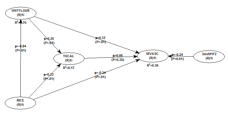
All of the results reported here are from analyses conducted using WarpPLS (). Below is the model with the main results of the analyses. (Click on it to enlarge. Use the "CRTL" and "+" keys to zoom in, and CRTL" and "-" to zoom out.) The arrows explore associations between variables, which are shown within ovals. The meaning of each variable is the following: SexM1F2 = sex, with 1 assigned to males and 2 to females; MVASC = mortality from all cardiovascular diseases (ages 35-69); TKCAL = total calorie intake per day; WHTFLOUR = wheat flour intake (g/day); and RICE = and rice intake (g/day).

The variables to the left of MVASC are the main predictors of interest in the model. The one to the right is a control variable – SexM1F2. The path coefficients (indicated as beta coefficients) reflect the strength of the relationships. A negative beta means that the relationship is negative; i.e., an increase in a variable is associated with a decrease in the variable that it points to. The P values indicate the statistical significance of the relationship; a P lower than 0.05 generally means a significant relationship (95 percent or higher likelihood that the relationship is “real”).

In summary, the model above seems to be telling us that:

- As rice intake increases, wheat flour intake decreases significantly (beta=-0.84; P<0.01). This relationship would be the same if the arrow pointed in the opposite direction. It suggests that there is a sharp divide between rice-consuming and wheat flour-consuming regions.

- As wheat flour intake increases, mortality from all cardiovascular diseases increases significantly (beta=0.32; P<0.01). This is after controlling for the effects of rice and total calorie intake. That is, wheat flour seems to have some inherent properties that make it bad for one’s health, even if one doesn’t consume that many calories.

- As rice intake increases, mortality from all cardiovascular diseases decreases significantly (beta=-0.24; P<0.01). This is after controlling for the effects of wheat flour and total calorie intake. That is, this effect is not entirely due to rice being consumed in place of wheat flour. Still, as you’ll see later in this post, this relationship is nonlinear. Excessive rice intake does not seem to be very good for one’s health either.

- Increases in wheat flour and rice intake are significantly associated with increases in total calorie intake (betas=0.25, 0.33; P<0.01). This may be due to wheat flour and rice intake: (a) being themselves, in terms of their own caloric content, main contributors to the total calorie intake; or (b) causing an increase in calorie intake from other sources. The former is more likely, given the effect below.

- The effect of total calorie intake on mortality from all cardiovascular diseases is insignificant when we control for the effects of rice and wheat flour intakes (beta=0.08; P=0.35). This suggests that neither wheat flour nor rice exerts an effect on mortality from all cardiovascular diseases by increasing total calorie intake from other food sources.

- Being female is significantly associated with a reduction in mortality from all cardiovascular diseases (beta=-0.24; P=0.01). This is to be expected. In other words, men are women with a few design flaws, so to speak. (This situation reverses itself a bit after menopause.)

Wheat flour displaces rice

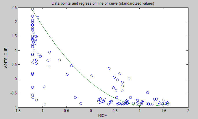
The graph below shows the shape of the association between wheat flour intake (WHTFLOUR) and rice intake (RICE). The values are provided in standardized format; e.g., 0 is the mean (a.k.a. average), 1 is one standard deviation above the mean, and so on. The curve is the best-fitting U curve obtained by the software. It actually has the shape of an exponential decay curve, which can be seen as a section of a U curve. This suggests that wheat flour consumption has strongly displaced rice consumption in several regions in China, and also that wherever rice consumption is high wheat flour consumption tends to be low.

As wheat flour intake goes up, so does cardiovascular disease mortality

The graphs below show the shapes of the association between wheat flour intake (WHTFLOUR) and mortality from all cardiovascular diseases (MVASC). In the first graph, the values are provided in standardized format; e.g., 0 is the mean (or average), 1 is one standard deviation above the mean, and so on. In the second graph, the values are provided in unstandardized format and organized in terciles (each of three equal intervals).

The curve in the first graph is the best-fitting U curve obtained by the software. It is a quasi-linear relationship. The higher the consumption of wheat flour in a county, the higher seems to be the mortality from all cardiovascular diseases. The second graph suggests that mortality in the third tercile, which represents a consumption of wheat flour of 501 to 751 g/day (a lot!), is 69 percent higher than mortality in the first tercile (0 to 251 g/day).

Rice seems to be protective, as long as intake is not too high

The graphs below show the shapes of the association between rice intake (RICE) and mortality from all cardiovascular diseases (MVASC). In the first graph, the values are provided in standardized format. In the second graph, the values are provided in unstandardized format and organized in terciles.

Here the relationship is more complex. The lowest mortality is clearly in the second tercile (206 to 412 g/day). There is a lot of variation in the first tercile, as suggested by the first graph with the U curve. (Remember, as rice intake goes down, wheat flour intake tends to go up.) The U curve here looks similar to the exponential decay curve shown earlier in the post, for the relationship between rice and wheat flour intake.

In fact, the shape of the association between rice intake and mortality from all cardiovascular diseases looks a bit like an “echo” of the shape of the relationship between rice and wheat flour intake. Here is what is creepy. This echo looks somewhat like the first curve (between rice and wheat flour intake), but with wheat flour intake replaced by “death” (i.e., mortality from all cardiovascular diseases).

What does this all mean?

- Wheat flour displacing rice does not look like a good thing. Wheat flour intake seems to have strongly displaced rice intake in the counties where it is heavily consumed. Generally speaking, that does not seem to have been a good thing. It looks like this is generally associated with increased mortality from all cardiovascular diseases.

- High glycemic index food consumption does not seem to be the problem here. Wheat flour and rice have very similar glycemic indices (but generally not glycemic loads; see below). Both lead to blood glucose and insulin spikes. Yet, rice consumption seems protective when it is not excessive. This is true in part (but not entirely) because it largely displaces wheat flour. Moreover, neither rice nor wheat flour consumption seems to be significantly associated with cardiovascular disease via an increase in total calorie consumption. This is a bit of a blow to the theory that high glycemic carbohydrates necessarily cause obesity, diabetes, and eventually cardiovascular disease.

- The problem with wheat flour is … hard to pinpoint, based on the results summarized here. Maybe it is the fact that it is an ultra-refined carbohydrate-rich food; less refined forms of wheat could be healthier. In fact, the glycemic loads of less refined carbohydrate-rich foods tend to be much lower than those of more refined ones (). (Also, boiled brown rice has a glycemic load that is about three times lower than that of whole wheat bread; whereas the glycemic indices are about the same.) Maybe the problem is wheat flour's  gluten content. Maybe it is a combination of various factors (), including these.

Notes

- The path coefficients (indicated as beta coefficients) reflect the strength of the relationships; they are a bit like standard univariate (or Pearson) correlation coefficients, except that they take into consideration multivariate relationships (they control for competing effects on each variable). Whenever nonlinear relationships were modeled, the path coefficients were automatically corrected by the software to account for nonlinearity.

- The software used here identifies non-cyclical and mono-cyclical relationships such as logarithmic, exponential, and hyperbolic decay relationships. Once a relationship is identified, data values are corrected and coefficients calculated. This is not the same as log-transforming data prior to analysis, which is widely used but only works if the underlying relationship is logarithmic. Otherwise, log-transforming data may distort the relationship even more than assuming that it is linear, which is what is done by most statistical software tools.

- The R-squared values reflect the percentage of explained variance for certain variables; the higher they are, the better the model fit with the data. In complex and multi-factorial phenomena such as health-related phenomena, many would consider an R-squared of 0.20 as acceptable. Still, such an R-squared would mean that 80 percent of the variance for a particularly variable is unexplained by the data.

- The P values have been calculated using a nonparametric technique, a form of resampling called jackknifing, which does not require the assumption that the data is normally distributed to be met. This and other related techniques also tend to yield more reliable results for small samples, and samples with outliers (as long as the outliers are “good” data, and are not the result of measurement error).

- Only two data points per county were used (for males and females). This increased the sample size of the dataset without artificially reducing variance, which is desirable since the dataset is relatively small. This also allowed for the test of commonsense assumptions (e.g., the protective effects of being female), which is always a good idea in a complex analysis because violation of commonsense assumptions may suggest data collection or analysis error. On the other hand, it required the inclusion of a sex variable as a control variable in the analysis, which is no big deal.

- Since all the data was collected around the same time (late 1980s), this analysis assumes a somewhat static pattern of consumption of rice and wheat flour. In other words, let us assume that variations in consumption of a particular food do lead to variations in mortality. Still, that effect will typically take years to manifest itself. This is a major limitation of this dataset and any related analyses.

- Mortality from schistosomiasis infection (MSCHIST) does not confound the results presented here. Only counties where no deaths from schistosomiasis infection were reported have been included in this analysis. Mortality from all cardiovascular diseases (MVASC) was measured using the variable M059 ALLVASCc (ages 35-69).

The China Study II: Cholesterol seems to protect against cardiovascular disease

First of all, many thanks are due to Dr. Campbell and his collaborators for collecting and compiling the data used in this analysis. The data has been compliled by those researchers to disseminate the data from a study often referred to as the “China Study II”. It has already been analyzed by other bloggers. Notable analyses have been conducted by Ricardo at Canibais e Reis, Stan at Heretic, and Denise at Raw Food SOS.

The analyses in this post differ from those other analyses in various aspects. One of them is that data for males and females were used separately for each county, instead of the totals per county. Only two data points per county were used (for males and females). This increased the sample size of the dataset without artificially reducing variance (for more details, see “Notes” at the end of the post), which is desirable since the dataset is relatively small. This also allowed for the test of commonsense assumptions (e.g., the protective effects of being female), which is always a good idea in a complex analysis because violation of commonsense assumption may suggest data collection or analysis error. On the other hand, it required the inclusion of a sex variable as a control variable in the analysis, which is no big deal.

The analysis was conducted using WarpPLS. Below is the model with the main results of the analysis. (Click on it to enlarge. Use the "CRTL" and "+" keys to zoom in, and CRTL" and "-" to zoom out.) The arrows explore associations between variables, which are shown within ovals. The meaning of each variable is the following: SexM1F2 = sex, with 1 assigned to males and 2 to females; HDLCHOL = HDL cholesterol; TOTCHOL = total cholesterol; MSCHIST = mortality from schistosomiasis infection; and MVASC = mortality from all cardiovascular diseases.

The variables to the left of MVASC are the main predictors of interest in the model – HDLCHOL and TOTCHOL. The ones to the right are control variables – SexM1F2 and MSCHIST. The path coefficients (indicated as beta coefficients) reflect the strength of the relationships. A negative beta means that the relationship is negative; i.e., an increase in a variable is associated with a decrease in the variable that it points to. The P values indicate the statistical significance of the relationship; a P lower than 0.05 generally means a significant relationship (95 percent or higher likelihood that the relationship is “real”).

In summary, this is what the model above is telling us:

- As HDL cholesterol increases, total cholesterol increases significantly (beta=0.48; P<0.01). This is to be expected, as HDL is a main component of total cholesterol, together with VLDL and LDL cholesterol.

- As total cholesterol increases, mortality from all cardiovascular diseases decreases significantly (beta=-0.25; P<0.01). This is to be expected if we assume that total cholesterol is in part an intervening variable between HDL cholesterol and mortality from all cardiovascular diseases. This assumption can be tested through a separate model (more below). Also, there is more to this story, as noted below.

- The effect of HDL cholesterol on mortality from all cardiovascular diseases is nonsignificant when we control for the effect of total cholesterol (beta=-0.08; P=0.26). This suggests that HDL’s protective role is subsumed by the variable total cholesterol, and also that it is possible that there is something else associated with total cholesterol that makes it protective. Otherwise the effect of total cholesterol might have been nonsignificant, and the effect of HDL cholesterol significant (the reverse of what we see here).

- Being female is significantly associated with a reduction in mortality from all cardiovascular diseases (beta=-0.16; P=0.01). This is to be expected. In other words, men are women with a few design flaws. (This situation reverses itself a bit after menopause.)

- Mortality from schistosomiasis infection is significantly and inversely associated with mortality from all cardiovascular diseases (beta=-0.28; P<0.01). This is probably due to those dying from schistosomiasis infection not being entered in the dataset as dying from cardiovascular diseases, and vice-versa.

Two other main components of total cholesterol, in addition to HDL cholesterol, are VLDL and LDL cholesterol. These are carried in particles, known as lipoproteins. VLDL cholesterol is usually represented as a fraction of triglycerides in cholesterol equations (e.g., the Friedewald and Iranian equations). It usually correlates inversely with HDL; that is, as HDL cholesterol increases, usually VLDL cholesterol decreases. Given this and the associations discussed above, it seems that LDL cholesterol is a good candidate for the possible “something else associated with total cholesterol that makes it protective”. But waidaminet! Is it possible that the demon particle, the LDL, serves any purpose other than giving us heart attacks?

The graph below shows the shape of the association between total cholesterol (TOTCHOL) and mortality from all cardiovascular diseases (MVASC). The values are provided in standardized format; e.g., 0 is the average, 1 is one standard deviation above the mean, and so on. The curve is the best-fitting S curve obtained by the software (an S curve is a slightly more complex curve than a U curve).

The graph below shows some of the data in unstandardized format, and organized differently. The data is grouped here in ranges of total cholesterol, which are shown on the horizontal axis. The lowest and highest ranges in the dataset are shown, to highlight the magnitude of the apparently protective effect. Here the two variables used to calculate mortality from all cardiovascular diseases (MVASC; see “Notes” at the end of this post) were added. Clearly the lowest mortality from all cardiovascular diseases is in the highest total cholesterol range, 172.5 to 180; and the highest mortality in the lowest total cholesterol range, 120 to 127.5. The difference is quite large; the mortality in the lowest range is approximately 3.3 times higher than in the highest.

The shape of the S-curve graph above suggests that there are other variables that are confounding the results a bit. Mortality from all cardiovascular diseases does seem to generally go down with increases in total cholesterol, but the smooth inflection point at the middle of the S-curve graph suggests a more complex variation pattern that may be influenced by other variables (e.g., smoking, dietary patterns, or even schistosomiasis infection; see “Notes” at the end of this post).

As mentioned before, total cholesterol is strongly influenced by HDL cholesterol, so below is the model with only HDL cholesterol (HDLCHOL) pointing at mortality from all cardiovascular diseases (MVASC), and the control variable sex (SexM1F2).

The graph above confirms the assumption that HDL’s protective role is subsumed by the variable total cholesterol. When the variable total cholesterol is removed from the model, as it was done above, the protective effect of HDL cholesterol becomes significant (beta=-0.27; P<0.01). The control variable sex (SexM1F2) was retained even in this targeted HDL effect model because of the expected confounding effect of sex; females generally tend to have higher HDL cholesterol and less cardiovascular disease than males.

Below, in the “Notes” section (after the “Reference”) are several notes, some of which are quite technical. Providing them separately hopefully has made the discussion above a bit easier to follow. The notes also point at some limitations of the analysis. This data needs to be analyzed from different angles, using multiple models, so that firmer conclusions can be reached. Still, the overall picture that seems to be emerging is at odds with previous beliefs based on the same dataset.

What could be increasing the apparently protective HDL and total cholesterol in this dataset? High consumption of animal foods, particularly foods rich in saturated fat and cholesterol, are strong candidates. Low consumption of vegetable oils rich in linoleic acid, and of foods rich in refined carbohydrates, are also good candidates. Maybe it is a combination of these.

We need more analyses!


Notes:

- The path coefficients (indicated as beta coefficients) reflect the strength of the relationships; they are a bit like standard univariate (or Pearson) correlation coefficients, except that they take into consideration multivariate relationships (they control for competing effects on each variable).

- The R-squared values reflect the percentage of explained variance for certain variables; the higher they are, the better the model fit with the data. In complex and multi-factorial phenomena such as health-related phenomena, many would consider an R-squared of 0.20 as acceptable. Still, such an R-squared would mean that 80 percent of the variance for a particularly variable is unexplained by the data.

- The P values have been calculated using a nonparametric technique, a form of resampling called jackknifing, which does not require the assumption that the data is normally distributed to be met. This and other related techniques also tend to yield more reliable results for small samples, and samples with outliers (as long as the outliers are “good” data, and are not the result of measurement error).

- Colinearity is an important consideration in models that analyze the effect of multiple predictors on one single variable. This is particularly true for multiple regression models, where there is a temptation of adding many predictors to the model to see which ones come out as the “winners”. This often backfires, as colinearity can severely distort the results. Some multiple regression techniques, such as automated stepwise regression with backward elimination, are particularly vulnerable to this problem. Colinearity is not the same as correlation, and thus is defined and measured differently. Two predictor variables may be significantly correlated and still have low colinearity. A reasonably reliable measure of colinearity is the variance inflation factor. Colinearity was tested in this model, and was found to be low.

- An effort was made here to avoid multiple data points per county (even though this was available for some variables), because this could artificially reduce the variance for each variable, and potentially bias the results. The reason for this is that multiple answers from a single county would normally be somewhat correlated; a higher degree of intra-county correlation than inter-county correlation. The resulting bias would be difficult to control for, via one or more control variables. With only two data points per county, one for males and the other for females, one can control for intra-country correlation by adding a “dummy” sex variable to the analysis, as a control variable. This was done here.

- Mortality from schistosomiasis infection (MSCHIST) is a variable that tends to affect the results in a way that makes it more difficult to make sense of them. Generally this is true for any infectious diseases that significantly affect a population under study. The problem with infection is that people with otherwise good health or habits may get the infection, and people with bad health and habits may not. Since cholesterol is used by the human body to fight disease, it may go up, giving the impression that it is going up for some other reason. Perhaps instead of controlling for its effect, as done here, it would have been better to remove from the analysis those counties with deaths from schistosomiasis infection. (See also this post, and this one.)

- Different parts of the data were collected at different times. It seems that the mortality data is for the period 1986-88, and the rest of the data is for 1989. This may have biased the results somewhat, even though the time lag is not that long, especially if there were changes in certain health trends from one period to the other. For example, major migrations from one county to another could have significantly affected the results.

- The following measures were used, from the China Study II dataset, like the other measures. P002 HDLCHOL, for HDLCHOL; P001 TOTCHOL, for TOTCHOL; and M021 SCHISTOc, for MSCHIST.

- SexM1F2 is a “dummy” variable that was coded with 1 assigned to males and 2 to females. As such, it essentially measures the “degree of femaleness” of the respondents. Being female is generally protective against cardiovascular disease, a situation that reverts itself a bit after menopause.

- MVASC is a composite measure of the two following variables, provided as component measures of mortality from all cardiovascular diseases: M058 ALLVASCb (ages 0-34), and M059 ALLVASCc (ages 35-69). A couple of obvious problems: (a) they does not include data on people older than 69; and (b) they seem to capture a lot of diseases, including some that do not seem like typical cardiovascular diseases. A factor analysis was conducted, and the loadings and cross-loadings suggested good validity. Composite reliability was also good. So essentially MVASC is measured here as a “latent variable” with two “indicators”. Why do this? The reason is that it reduces the biasing effects of incomplete data and measurement error (e.g., exclusion of folks older than 69). By the way, there is always some measurement error in any dataset.

- This note is related to measurement error in connection with the indicators for MVASC. There is something odd about the variables M058 ALLVASCb (ages 0-34), and M059 ALLVASCc (ages 35-69). According to the dataset, mortality from cardiovascular diseases for ages 0-34 is typically higher than for 35-69, for many counties. Given the good validity and reliability for MVASC as a latent variable, it is possible that the values for these two indicator variables were simply swapped by mistake.

Is heavy physical activity a major trigger of death by sudden cardiac arrest? Not in Oregon

The idea that heavy physical activity is a main trigger of heart attacks is widespread. Often endurance running and cardio-type activities are singled out. Some people refer to this as “death by running”.

Good cardiology textbooks, such as the Mayo Clinic Cardiology, tend to give us a more complex and complete picture. So do medical research articles that report on studies of heart attacks based on comprehensive surveys.

Reddy and colleagues (2009) studied sudden cardiac arrest events followed by death from 2002 to 2005 in Multnomah County in Oregon. This study was part of the ongoing Oregon Sudden Unexpected Death Study. Multnomah County has an area of 435 square miles, and had a population of over 677 thousand at the time of the study. The full reference to the article and a link to a full-text version are at the end of this post.

The researchers grouped deaths by sudden cardiac arrests (SCAs) according to the main type of activity being performed before the event. Below is how the authors defined the activities, quoted verbatim from the article. MET is a measure of the amount of energy spent in the activity; one MET is the amount of energy spent by a person sitting quietly.

- Sleep (MET 0.9): subjects who were sleeping when they sustained SCA.
- Light activity (MET 1.0–3.4): included bathing, dressing, cooking, cleaning, feeding, household walking and driving.
- Moderate activity (MET 3.5–5.9): included walking for exercise, mowing lawn, gardening, working in the yard, dancing.
- Heavy activity (MET score ≥6): included sports such as tennis, running, jogging, treadmill, skiing, biking.
- Sexual activity (MET score 1.3): included acts of sexual intercourse.

What did they find? Not what many people would expect.

The vast majority of the people dying of sudden cardiac arrest were doing things that fit the “light activity” group above prior to their death. This applies to both genders. The figure below (click to enlarge) shows the percentages of men and women who died from sudden cardiac arrest, grouped by activity type.

Sudden cardiac arrests were also categorized as witnessed or un-witnessed. For witnessed, someone saw them happening. For un-witnessed, the person was seen alive, and within 24 hours had died. So the data for witnessed sudden cardiac arrests is a bit more reliable. The table below displays the distribution of mean age, gender and known coronary artery disease (CAD) in those with witnessed sudden cardiac arrest.

Look at the bottom row, showing those with known coronary artery disease. Again, light activity is the main trigger. Sleep comes second. The numbers within parentheses refer to percentages within each activity group. Those percentages are not very helpful in the identification of the most important triggers, although they do suggest that coronary artery disease is a major risk factor. For example, among those who died from sudden cardiac arrest while having sex, 57 percent had known coronary artery disease. For light activity, 36 percent had known coronary artery disease.

As a caveat, it is worth noting that heavy activity appears to be more of a trigger in younger individuals than in older ones. This may simply reflect the patterns of activities at different ages. However, this does not seem to properly account for the large differences observed in triggers; the standard deviation for age in the heavy activity group was large enough to include plenty of seniors. Still, it would have been nice to see a multivariate analysis controlling for various effects, including age.

So what is going on here?

The authors give us a hint. The real culprit may be bottled up emotional stress and sleep disorders; the latter may be caused by stress, as well as by obesity and other related problems. They have some data that points in those directions. That makes some sense.

We humans have evolved “fight-or-flight” mechanisms that involve large hormonal discharges in response to stressors. Our ancestors needed those. For example, they needed those to either fight or run for their lives in response to animal attacks.

Modern humans experience too many stressors while sitting down, as in stressful car commutes and nasty online interactions. The stresses cause “fight-or-flight” hormonal discharges, but are followed by neither “fight” nor “flight” in most cases. This cannot be very good for us.

Death by running!? More like death by not running!

Reference:

Reddy, P.R., Reinier, K., Singh, T., Mariani, R., Gunson, K., Jui, J., & Chugh, S.S. (2009). Physical activity as a trigger of sudden cardiac arrest: The Oregon Sudden Unexpected Death Study. International Journal of Cardiology, 131(3), 345–349.

Total cholesterol and cardiovascular disease: A U-curve relationship

The hypothesis that blood cholesterol levels are positively correlated with heart disease (the lipid hypothesis) dates back to Rudolph Virchow in the mid-1800s.

One famous study that supported this hypothesis was Ancel Keys's Seven Countries Study, conducted between the 1950s and 1970s. This study eventually served as the foundation on which much of the advice that we receive today from doctors is based, even though several other studies have been published since that provide little support for the lipid hypothesis.

The graph below (from O Primitivo) shows the results of one study, involving many more countries than Key's Seven Countries Study, that actually suggests a NEGATIVE linear correlation between total cholesterol and cardiovascular disease.

Now, most relationships in nature are nonlinear, with quite a few following a pattern that looks like a U-curve (plain or inverted); sometimes called a J-curve pattern. The graph below (also from O Primitivo) shows the U-curve relationship between total cholesterol and mortality, with cardiovascular disease mortality indicated through a dotted red line at the bottom.

This graph has been obtained through a nonlinear analysis, and I think it provides a better picture of the relationship between total cholesterol (TC) and mortality. Based on this graph, the best range of TC that one can be at is somewhere between 210, where cardiovascular disease mortality is minimized; and 220, where total mortality is minimized.

The total mortality curve is the one indicated through the full blue line at the top. In fact, it suggests that mortality increases sharply as TC decreases below 200.

Now, these graphs relate TC with disease and mortality, and say nothing about LDL cholesterol (LDL). In my own experience, and that of many people I know, a TC of about 200 will typically be associated with a slightly elevated LDL (e.g., 110 to 150), even if one has a high HDL cholesterol (i.e., greater than 60).

Yet, most people who have a LDL greater than 100 will be told by their doctors, usually with the best of the intentions, to take statins, so that they can "keep their LDL under control". (LDL levels are usually calculated, not measured directly, which itself creates a whole new set of problems.)

Alas, reducing LDL to 100 or less will typically reduce TC below 200. If we go by the graphs above, especially the one showing the U-curves, these folks' risk for cardiovascular disease and mortality will go up - exactly the opposite effect that they and their doctors expected. And that will cost them financially as well, as statin drugs are expensive, in part to pay for all those TV ads.

Want to improve your cholesterol profile? Replace refined carbs and sugars with saturated fat and cholesterol in your diet

An interesting study by Clifton and colleagues (1998; full reference and link at the end of this post) looked at whether LDL cholesterol particle size distribution at baseline (i.e., beginning of the study) for various people was a determinant of lipid profile changes in each of two diets – one low and the other high in fat. This study highlights a few interesting points made in a previous post, which are largely unrelated to the main goal or findings of the study, but that are supported by side findings:

- As one increases dietary cholesterol and fat consumption, particularly saturated fat, circulating HDL cholesterol increases significantly. This happens whether one is taking niacin or not, although niacin seems to help, possibly as an independent (not moderating) factor. Increasing serum vitamin D levels, which can be done through sunlight exposure and supplementation, are also known to increase circulating HDL cholesterol.

- As one increases dietary cholesterol and fat consumption, particularly saturated fat, triglycerides in the fasting state (i.e., measured after a 8-hour fast) decrease significantly, particularly on a low carbohydrate diet. Triglycerides in the fasting state are negatively correlated with HDL cholesterol; they go down as HDL cholesterol goes up. This happens whether one is taking niacin or supplementing omega 3 fats or not, although these seem to help, possibly as independent factors.

- If one increases dietary fat intake, without also decreasing carbohydrate intake (particularly in the form of refined grains and sugars), LDL cholesterol will increase. Even so, LDL particle sizes will shift to more benign forms, which are the larger forms. Not all LDL particles change to benign forms, and there seem to be some genetic factors that influence this. LDL particles larger than 26 nm in diameter simply cannot pass through the gaps in the endothelium, which is a thin layer of cells lining the interior surface of arteries, and thus do not induce plaque formation.

The study by Clifton and colleagues (1998) involved 54 men and 51 women with a wide range of lipid profiles. They first underwent a 2-week low fat period, after which they were given two liquid supplements in addition to their low fat diet, for a period of 3 weeks. One of the liquid supplements contained 31 to 40 g of fat, and 650 to 845 mg of cholesterol. The other was fat and cholesterol free.

Studies that adopt a particular diet at baseline have the advantage of departing from a uniform diet across conditions. They also typically have one common characteristic: the baseline diet reflects the beliefs of the authors about what an ideal diet is. That is not always the case, of course. If this was indeed the case here, we have a particularly interesting study, because in that case the side findings discussed below contradicted the authors’ beliefs.

The table below shows the following measures for the participants in the study: age, body mass index (BMI), waist-to-hip ratio (WHR), total cholesterol, triglycerides, low-density lipoprotein (LDL) cholesterol, and three subtypes of high-density lipoprotein (HDL) cholesterol. LDL cholesterol is the colloquially known as the “bad” type, and “HDL” as the good one (which is an oversimplification). In short, the participants were overweight, middle-aged men and women, with relatively poor lipid profiles.

At the bottom of the table is the note “P < 0.001”, following a small “a”. This essentially means that on the rows indicated by an “a”, like the “WHR” row, the difference in the averages (e.g., 0.81 for women, and 0.93 for men, in the WHR row) was significantly different from what one would expect it to be due to chance alone. More precisely, the likelihood that the difference was due to chance was lower than 0.001, or 0.1 percent, in the case of a P < 0.001. Usually a difference between averages (a.k.a. means) associated with a P < 0.05 will be considered statistically significant.

Since the LDL cholesterol concentrations (as well as other lipoprotein concentrations) are listed on the table in mmol/L, and many people receive those measures in mg/dL in blood lipid profile test reports, below is a conversion table for LDL cholesterol (from: Wikipedia).

The table below shows the dietary intake in the low and high fat diets. Note that in the high fat diet, not only is the fat intake higher, but so is the cholesterol intake. The latter is significantly higher, more than 4 times the intake in the low fat diet, and about 2.5 times the recommended daily value by the U.S. Food and Drug Administration. The total calorie intake is reported as slightly lower in the high fat diet than in the low fat diet.

Note that the largest increase was in saturated fat, followed by an almost equally large increase in monounsaturated fat. This, together with the increase in cholesterol, mimics a move to a diet where fatty meat and organs are consumed in higher quantities, with a corresponding reduction in the intake of refined carbohydrates (e.g., bread, pasta, sugar, potatoes) and lean meats.

Finally, the table below shows the changes in lipid profiles in the low and high fat diets. Note that all subtypes of HDL (or "good") cholesterol concentrations were significantly higher in the high fat diet, which is very telling, because HDL cholesterol concentrations are much better predictors of cardiovascular disease than LDL or total cholesterol concentrations. The higher the HDL cholesterol, the lower the risk of cardiovascular disease.

In the table above, we also see that triglycerides are significantly lower in the high fat diet, which is also good, because high fasting triglyceride concentrations are associated with cardiovascular disease and also insulin resistance (which is associated with diabetes).

However, the total and LDL cholesterol were also significantly higher in the high fat compared to the low fat diet. Is this as bad as it sounds? Not when we look at other factors that are not clear from the tables in the article.

One of those factors is the likely change in LDL particle size. LDL particle sizes almost always increase with significant increases in HDL; frequently going up in diameter beyond 26 nm, and thus passing the threshold beyond which an LDL particle can penetrate the endothelium and help form a plaque.

Another important factor to take into consideration is the somewhat strange decision by the authors to use the Friedewald equation to estimate the LDL concentrations in the low and high fat diets. Through the Friedewald equation, LDL is calculated as follows (where TC is total cholesterol):

    LDL = TC – HDL – Triglycerides / 5

Here is one of the problems with the Friedewald equation. Let us assume that an individual has the following lipid profile numbers: TC = 200, HDL = 50, and trigs. = 150. The calculated LDL will be 120. Let us assume that this same individual reduces trigs. to 50, from the previous 150, keeping all of the other measures constant. This is a major improvement. Yet, the calculated LDL will now be 140, and a doctor will tell this person to consider taking statins!

By the way, most people who do a blood test and get their lipid profile report also get their LDL calculated through the Friedewald equation. Usually this is indicated through a "CALC" note next to the description of the test or the calculated LDL number.

Finally, total cholesterol is not a very useful measure, because an elevated total cholesterol may be primarily reflecting an elevated HDL, which is healthy. Also, a slightly elevated total cholesterol seems to be protective, as it is associated with reduced overall mortality and also reduced mortality from cardiovascular disease, according to U-curve regression studies comparing mortality and total cholesterol levels in different countries.

We do not know for sure that the participants in this study were consuming a lot of refined carbohydrates and/or sugars at baseline. But it is a safe bet that they were, since they were consuming 214 g of carbohydrates per day. It is difficult, although not impossible, to eat that many carbohydrates per day by eating only vegetables and fruits, which are mostly water. Consumption of starches makes it easier to reach that level.

This is why when one goes on a paleo diet, he or she reduces significantly the amount of dietary carbohydrates; even more so on a targeted low carbohydrate diet, such as the Atkins diet. Richard K. Bernstein, who is a type 1 diabetic and has been adopting a strict low carbohydrate diet during most of his adult life, had the following lipid profile at 72 years of age: HDL = 118, LDL = 53, trigs. = 45. His fasting blood sugar was reportedly 83 mg/dl. Click here to listen to an interview with Dr. Bernstein on the The Livin' La Vida Low-Carb Show.

The lipid profile improvement observed (e.g., a 14 percent increase in HDL from baseline for men, and about half that for women, in only 3 weeks) was very likely due to an increase in dietary saturated fat and cholesterol combined with a decrease in refined carbohydrates and sugars. The improvement would probably have been even more impressive with a higher increase in saturated fat, as long as it was accompanied by the elimination of refined carbohydrates and sugars from the participants’ diets.

Reference:

Clifton, P. M., M. Noakes, and P. J. Nestel (1998). LDL particle size and LDL and HDL cholesterol changes with dietary fat and cholesterol in healthy subjects. J. Lipid. Res. 39: 1799–1804.

The PCSK9 enzyme, LDL cholesterol, and cardiovascular diseases

Cardiovascular diseases are currently the leading cause of death in most developed countries. They are particularly common among seniors; i.e., those aged 65 and older. Part of the reason for this is that infectious diseases do not kill as many people as they used to.

Given the trend toward population aging, with seniors making up an increasingly larger percentage of the population, the market for drugs against cardiovascular diseases is growing. A new class of such drugs is making the news lately; they target the PCSK9 enzyme ().

Enzymes are (usually) proteins that speed up chemical reactions, and are needed in virtually all metabolic processes that occur in cells. Proprotein convertase subtilisin/kexin type 9 (PCSK9) is an enzyme that degrades LDL cholesterol receptors on the surface of liver cells. Fewer LDL cholesterol receptors mean reduced uptake of the particles that carry LDL cholesterol, and thus more LDL particles in circulation. This may be problematic if these are small-dense LDL particles ().

Small-dense LDL particles include particles that are significantly smaller than the gaps in the endothelium (). The endothelium is a thin layer of cells that line the interior of arteries. Those gaps are about 25-26 nanometers (nm) in diameter. Small-dense LDL particles can contribute a lot more to the formation of atheromas (atherosclerotic plaques) in predisposed individuals than large-buoyant LDL particles.

There is evidence of the natural occurrence of low LDL cholesterol in individuals of African descent due to genetic mutations influencing PCSK9 levels (). This leads us to a very important question. By reducing PCSK9 in circulation, can we also reduce the incidence of cardiovascular disease?

The answer to this question depends on whether LDL cholesterol is a causative factor in cardiovascular disease. If it is, then reducing PCSK9 in circulation can indeed reduce the incidence of cardiovascular disease. The problem is that, most of the evidence so far suggests that LDL cholesterol is NOT a causative factor in cardiovascular disease.

Yes, there are studies that show that LDL cholesterol is correlated with cardiovascular disease, but the problem is that LDL cholesterol is a marker of other factors that are better candidates for causes of cardiovascular disease – hence the correlation. For example, LDL cholesterol goes up with mental stress (), and chronic mental stress seems to be a good candidate for a cause of cardiovascular disease.

LDL cholesterol is also a marker of a diet with more saturated fat in it (). In many contexts, a diet with more saturated fat in it is a more nutritious diet, which leads to a negative association between LDL cholesterol and mortality.

The graph below shows the shape of the association between total cholesterol (TOTCHOL) and mortality from all cardiovascular diseases (MVASC), based on an analysis of the China Study II dataset (). LDL cholesterol is the main component of total cholesterol in most people. The values are provided in standardized format; e.g., 0 is the average, 1 is one standard deviation above the mean, and so on. The best-fitting curve was obtained with the software WarpPLS ().

In fact, when we combine the totality of the evidence linking LDL cholesterol and cardiovascular diseases, LDL cholesterol seems to come out as a marker of protective factors. A reflection of this is a widely cited study by Weverling-Rijnsburger and colleagues, of LDL and HDL cholesterol as factors in cardiovascular diseases among people aged 85 and older (). The conclusions of the study were that:

- There was no association between LDL cholesterol level and risk of fatal cardiovascular disease.

- A low HDL cholesterol level was associated with a two-fold higher risk of fatal cardiovascular disease.

- Both low LDL cholesterol and low HDL cholesterol levels were associated with an increased mortality risk from infections.

The results above are particularly interesting because the study participants, given their ages, were at a high risk of mortality from cardiovascular diseases. It seems that the best scenario for these folks would have been a concomitant increase in both LDL and HDL cholesterol levels, which seems to be exactly what happens when one increases his or her intake of foods rich in saturated fat and dietary cholesterol ()!

Should you take a drug that targets the PCSK9 enzyme, to reduce your LDL cholesterol? Maybe you should ask Peter ().

Ischemic heart disease among Greenland Inuit: Data from 1962 to 1964

The traditional Inuit diet is very high in animal protein and fat. It also includes plant matter. Typically it is made up primarily of the following: fish, walrus, seal, whale, berries, and fireweed (of which syrups and jellies can be made).

Kjærgaard and colleagues (see under References, at the end of this post) examined data from an Inuit population in Greenland from 1962 to 1964, prior to the heavy westernization of their diet that is seen today. They investigated 96.9% of the whole population in three areas, including Ammassalik in East Greenland (n = 1,851).

Of those, only 181 adults, or 9.7 percent, had anything that looked like an abnormality that could suggest ischemia. This included ventricular hypertrophy (an enlargement of the heart chambers), leading to an overestimation because benign ventricular hypertrophy is induced by continuous physical exertion. These 181 adults were then selected for further screening.

Benign ventricular hypertrophy is also known as athlete's heart, because it is common among athletes. A prevalence of ventricular hypertrophy at a relatively young age, and declining with age, would suggest benign hypertrophy. The opposite would suggest pathological hypertrophy, which is normally induced by chronic hypertension.

As you can see from the figure below, from Kjærgaard et al. (2009), the pattern observed among the Inuit was of benign hypertrophy, suggestive of strong physical exertion at a young age.

A pattern of benign hypertrophy induced by robust physical activity is also consistent with reports by Stefansson (1958) about the life of the Eskimos in Northern Alaska. It is reasonable to assume that these Eskimos had a diet and lifestyle similar to the Greenland Inuit.

Back to Kjærgaard et al.’s (2009) study. The 181 adults selected for further screening then had a 12-lead ECG performed (this is a widely used test to check for heart abnormalities). The results suggested that only two men, aged 62 and 63 years, had ischemic heart disease. All in all, this suggests a prevalence of ischemic heart disease of 0.11 percent, which is very low.

(The authors of the article estimated the prevalence of ischemic heart disease at 1.1 percent, because they used the n = 181, as opposed to the original n = 1,851, in their calculation. The latter is the correct baseline sample size, in my opinion. Still, the authors present the 1.1 percent number as quite low as well, which it is.)

The prevalence of ischemic heart disease in the US of approximately 6.8 percent. That is, the prevalence in the US is 63 times higher than among the Inuit studied (using the 0.11 percent as the basis for comparison). And, it should be noted that there are many countries with a higher prevalence of ischemic heart disease than modern US.

It is possible that the low prevalence of ischemic heart disease among the Inuit was partly due to a higher mortality of those with the disease than in modern US, where medical intervention can prolong one's life in the presence of almost any disease. That is, perhaps many of those Inuit with ischemia would die quickly, and thus would not be captured by a study like this.

It is doubtful, however, that this would explain a difference as large as the one observed. Moreover, if many Inuit were dying due to ischemia, there would probably be plenty of evidence suggesting that. (I would imagine that the mysterious deaths associated with chest pain, and other related symptoms, would be a constant topic of conversation.) Reports from early explorers, however, suggest the opposite (e.g., Stefansson, 1958), and are consistent with the study described here.

In conclusion, this study suggests that the diet and lifestyle of the Greenland Inuit prior to the 1960’s (i.e., not their traditional diet and lifestyle, but approaching it) could be seen today as heart-healthy (at least for them), even though the Greenland Inuit ate a lot of animal protein and fat.

References:

Kjærgaard, M., Andersen, S., Holten, M., Mulvad, G., Kjærgaard, J.J. (2009). Low occurrence of ischemic heart disease among Inuit around 1963 suggested from ECG among 1851 East Greenland Inuit. Atherosclerosis, 203(2), 599-603.

Stefansson, V. (1958). Eskimo longevity in Northern Alaska. Science, 127(3288), 16-19.

What is “relative risk” (RR)? The case of alcohol frequency and its impact on mortality from stroke

This post is in response to an inquiry by Ivor (sorry for the delayed response). It refers to a recent study by Rantakömi and colleagues on the effect of alcohol consumption frequency on mortality from stroke (). The study followed men who consumed alcohol to different degrees, including no consumption at all, over a period of a little more than 20 years.

The study purportedly controlled for systolic blood pressure, smoking, body mass index, diabetes, socioeconomic status, and total amount of alcohol consumption. That is, its results are presented as holding regardless of those factors.

The main results were reported in terms of “relative risk” (RR) ratios. Here they are, quoted from the abstract:

“0.71 (95% CI, 0.30–1.68; P = 0.437) for men with alcohol consumption <0.5 times per week and 1.16 (95% CI, 0.54–2.50; P = 0.704) among men who consumed alcohol 0.5–2.5 times per week. Among men who consumed alcohol >2.5 times per week compared with nondrinkers, RR was 3.03 (95% CI, 1.19–7.72; P = 0.020).”

Note the P values reported within parentheses. They are the probabilities that the results are due to chance and thus “not real”, or not due to actual effects. By convention, P values equal to or lower than 0.05 are considered statistically significant. In consequence, P values greater than 0.05 are seen as referring to effects that cannot be unequivocally considered real.

This means that, of the results reported, only one seems to be due to a real effect, and that is the one that: “Among men who consumed alcohol >2.5 times per week compared with nondrinkers, RR was 3.03 …”

Why the authors report the statistically non-significant results as if they were noteworthy is unclear to me.

Before we go any further, let us look at what “relative risk” (RR) means. RR is given by the following ratio:

(Probability of an event when exposed) / (Probability of an event when not exposed)

In the study by Rantakömi and colleagues, the event is death from stroke. The exposure refers to alcohol consumption at a certain level, compared to no alcohol consumption (no exposure).

Now, let us go back to the result regarding consumption of alcohol more than 2.5 times per week. That result sounds ominous. It is helpful to keep in mind that the study by Rantakömi and colleagues followed a total of 2609 men with no history of stroke, of whom only 66 died from stroke.

Consider the following scenario. Let us say that 1 person in a group of 1,000 people who consumed no alcohol died from stroke. Let us also say that 3 people in a group of 1,000 people who consumed alcohol more than 2.5 times per week died from stroke. Given this, the RR would be: (3/1,000) / (1/1,000) = 3.

One could say, based on this, that: “Consuming alcohol more than 2.5 times per week increases the risk of dying from stroke by 200%”. Based on the RR, this is technically correct. It is rather misleading nevertheless.

If you think that increasing sample size may help ameliorate the problem, think again. The RR would be the same if it was 3 people versus 1 person in 1,000,000 (one million). With these numbers, the RR would be even less credible, in my view.

This makes the findings by Rantakömi and colleagues look a lot less ominous, don’t you think? This post is not really about the study by Rantakömi and colleagues. It is about the following question, which is in the title of this post: What is “relative risk” (RR)?

Quite frankly, given what one sees in RR-based studies, the answer is arguably not far from this:

RR is a ratio used in statistical analysis that makes minute effects look enormous; the effects in question would not normally be noticed by anyone in real life, and may be due to chance after all.

The reason I say that the effects “may be due to chance after all” is that when effects are such that 1 event in 1,000 would make a big difference, a researcher would have to control for practically everything in order to rule out confounders.

If one single individual with a genetic predisposition toward death from stroke falls into the group that consumes more alcohol, falling in that group entirely by chance (or due to group allocation bias), the RR-based results would be seriously distorted.

This highlights one main problem with epidemiological studies in general, where RR is a favorite ratio to be reported. The problem is that epidemiological studies in general refer to effects that are tiny.

One way to put results in context and present them more “honestly” would be to provide more information to readers, such as graphs showing data points and unstandardized scales, like the one below. This graph is from a previous post on latitude and cancer rates in the USA (), and has been generated with the software WarpPLS ().

This graph clearly shows that, while there seems to be an association between latitude and cancer rates in the USA, the total variation in cancer rates in the sample is only of around 3 in 1,000. This graph also shows outliers (e.g., Alaska), which call for additional explanations.

As for the issue of alcohol consumption frequency and mortality, I leave you with the results of a 2008 study by Breslow and Graubard, with more citations and published in a more targeted journal ():

“Average volume obscured effects of quantity alone and frequency alone, particularly for cardiovascular disease in men where quantity and frequency trended in opposite directions.”

In other words, alcohol consumption in terms of volume (quantity multiplied by frequency) appears to matter much more than quantity or frequency alone. We can state this even more simply: drinking two bottles of whiskey in one sitting, but only once every two weeks, is not going to be good for you.

In the end, providing more information to readers so that they can place the results in context is a matter of scientific honesty.

The 2012 Atherosclerosis egg study: More smoking is associated with more plaque, unless you eat more eggs

I blogged before about the study by David Spence and colleagues, published online in July 2012 in the journal Atherosclerosis (). This study attracted a lot of media attention (e.g., ). The article is titled: “Egg yolk consumption and carotid plaque”. The study argues that “regular consumption of egg yolk should be avoided by persons at risk of cardiovascular disease”. It hints at egg yolks being unhealthy in general, possibly even more so than cigarettes.

I used the numbers in Table 2 of the article (only 5 rows of data, one per quintile; i.e., N=5) to conduct a type of analysis that is rarely if ever conducted in health studies – a moderating effects analysis. A previous blog post summarizes the results of one such analysis using WarpPLS (). It looked into the effect of the number of eggs consumed per week on the association between blood LDL cholesterol and plaque (carotid plaque). The conclusion, which is admittedly tentative due to the small sample (N=5), was that plaque decreased as LDL cholesterol increased with consumption of 2.3 eggs per week or more ().

Recently I ran an analysis on the moderating effect of number of eggs consumed per week on the association between cumulative smoking (measured in “pack years”) and plaque. As it turns out, if you fit a 3D surface to the five data points that you get for these three variables from Table 2 of the article, you end up with a relatively smooth surface. Below is a 3D plot of the 5 data points, followed by a best-fitting 3D surface (developed using an experimental algorithm).

Based on this best-fitting surface you could then generate a contour graph, shown below. The “lines” are called “isolines”. Each isoline refers to plaque values that are constant for a set of eggs per week and cumulative smoking combinations. Next to the isolines are the corresponding plaque values. The first impression is indeed that both egg consumption and smoking are causing plaque buildup, as plaque clearly increases as one moves toward the top-right corner of the graph.

But focus your attention on each individual isoline, one at a time. It is clear that plaque remains constant for increases in cumulative smoking, as long as egg consumption increases. Take for example the isoline that refers to 120 mm2 of plaque area. An increase in cumulative smoking from about 14.5 to 16 pack years leads to no increase in plaque if egg consumption goes up from about 2 to 2.3 eggs per week.

These within-isoline trends, which are fairly stable across isolines (they are all slanted to the right), clearly contradict the idea that eggs cause plaque buildup. So, why does plaque buildup seem to clearly increase with egg consumption? Here is a good reason: egg consumption is very strongly correlated with age, and plaque increases with age. The correlation is a whopping 0.916. And I am not talking about cumulative egg consumption, which the authors also measure, through a variable called “egg-yolk years”. No, I am talking about eggs per week. In this dataset, older folks were eating more eggs, period.

The correlation between plaque and age is even higher: 0.977. Given this, it makes sense to look at individual isolines. This would be analogous to what biostatisticians often call “adjusting for age”, or analyzing the effect of egg consumption on plaque buildup “keeping age constant”. A different technique is to “control for age”; this technique would be preferable had the correlations been lower (say, lower than 0.7), as collinearity levels might have been below acceptable thresholds.

The underlying logic of the “keeping age constant” technique is fairly sound in the face of such a high correlation, which would make “controlling for age” very difficult due to collinearity. When we “keep age constant”, the results point at egg consumption being protective among smokers.

But diehard fans of the idea that eggs are unhealthy could explain the results differently. Maybe egg consumption causes plaque to go up, but smoking has a protective effect. Again taking the isoline that refers to 120 mm2 of plaque area, these diehard fans could say that an increase in egg consumption from 2 to 2.3 eggs per week leads to no increase in plaque if cumulative smoking goes up from about 14.5 to 16 pack years.

Not too long ago I also blogged about a medical case study of a man who ate approximately 25 eggs (20 to 30) per day for over 15 years (probably well over), was almost 90 years old (88) when the case was published in the prestigious The New England Journal of Medicine, and was in surprisingly good health (). This man was not a smoker.

Perhaps if this man smoked 25 cigarettes per day, and ate no eggs, he would be in even better health eh!?

The anatomy of a VAP test report

The vertical auto profile (VAP) test is an enhanced lipid profile test. It has been proposed, as a more complete test that relies on direct measurement of previously calculated lipid measures. The VAP test is particularly known for providing direct measurements of LDL cholesterol, instead of calculating them through equations ().

At the time of this writing, a typical VAP test report would provide direct measures of the cholesterol content of LDL, Lp(a), IDL, HDL, and VLDL particles. It would also provide additional measures referred to as secondary risk factors, notably particle density patterns and apolipoprotein concentrations. Finally, it would provide a customized risk summary and some basic recommendations for treatment. Below is the top part of a typical VAP test report (from the company Atherotech), showing measures of the cholesterol content of various particles. LDL cholesterol is combined for four particle subtypes, the small-dense subtypes 4 and 3, and the large-buoyant subtypes 2 and 1. A breakdown by LDL particle subtype is provided later in the VAP report.

In the table above, HDL cholesterol is categorized in two subtypes, the small-dense subtype 2, and the large-buoyant subtype 3. Interestingly, most of the HDL cholesterol in the table is supposedly of the least protective subtype, which seems to be a common finding in the general population. VLDL cholesterol is categorized in a similar way. IDL stands for intermediate-density lipoprotein; this is essentially a VLDL particle that has given off some of its content, particularly its triglyceride (or fat) cargo, but still remains in circulation.

Lp(a) is a special subtype of the LDL particle that is purported to be associated with markedly atherogenic factors. Mainstream medicine generally considers Lp(a) particles themselves to be atherogenic, which is highly debatable. Among other things, cardiovascular disease (CVD) risk and Lp(a) concentration follow a J-curve pattern, and Lp(a)’s range of variation in humans is very large. A blog post by Peter (Hyperlipid) has a figure right at the top that illustrates the former J-curve assertion (). The latter fact, related to range of variation, generally leads to a rather wide normal distribution of Lp(a) concentrations in most populations; meaning that a large number of individuals tend to fall outside Lp(a)’s optimal range and still have a low risk of developing CVD.

Below is the middle part of a typical VAP report, showing secondary risk factors, such as particle density patterns and apolipoprotein concentrations. LDL particle pattern A is considered to be the most protective, supposedly because large-buoyant LDL particles are less likely to penetrate the endothelial gaps, which are about 25 nm in diameter. Apolipoproteins are proteins that bind to fats for their transport in lipoproteins, to be used by various tissues for energy; free fatty acids also need to bind to proteins, notably albumin, to be transported to tissues for use as energy. Redundant particles and processes are everywhere in the human body!

Below is the bottom part of a typical VAP report, providing a risk summary and some basic recommendations. One of the recommendations is “to lower” the LDL target from 130mg/dL to 100mg/dL due to the presence of the checked emerging risk factors on the right, under “Considerations”. What that usually means in practice is a recommendation to take drugs, especially statins, to reduce LDL cholesterol levels. A recent post here and the discussion under it suggest that this would be a highly questionable recommendation in the vast majority of cases ().

What do I think about VAP tests? I think that they are useful in that they provide a lot more information about one’s lipids than standard lipid profiles, and more information is better than less. On the other hand, I think that people should be very careful about what they do with that information. There are even more direct tests that I would recommend before a decision to take drugs is made (, ), if that decision is ever made at all.

Triglycerides, VLDL, and industrial carbohydrate-rich foods

Below are the coefficients of association calculated by HealthCorrelator for Excel (HCE) for user John Doe. The coefficients of association are calculated as linear correlations in HCE (). The focus here is on the associations between fasting triglycerides and various other variables. Take a look at the coefficient of association at the top, with VLDL cholesterol, indicated with a red arrow. It is a very high 0.999.

Whoa! What is this – 0.999! Is John Doe a unique case? No, this strong association between fasting triglycerides and VLDL cholesterol is a very common pattern among HCE users. The reason is simple. VLDL cholesterol is not normally measured directly, but typically calculated based on fasting triglycerides, by dividing the fasting triglycerides measurement by 5. And there is an underlying reason for that - fasting triglycerides and VLDL cholesterol are actually very highly correlated, based on direct measurements of these two variables.

But if VLDL cholesterol is calculated based on fasting triglycerides (VLDL cholesterol  = fasting triglycerides / 5), how come the correlation is 0.999, and not a perfect 1? The reason is the rounding error in the measurements. Whenever you see a correlation this high (i.e., 0.999), it is reasonable to suspect that the source is an underlying linear relationship disturbed by rounding error.

Fasting triglycerides are probably the most useful measures on standard lipid panels. For example, fasting triglycerides below 70 mg/dl suggest a pattern of LDL particles that is predominantly of large and buoyant particles. This pattern is associated with a low incidence of cardiovascular disease (). Also, chronically high fasting triglycerides are a well known marker of the metabolic syndrome, and a harbinger of type 2 diabetes.

Where do large and buoyant LDL particles come from? They frequently start as "big" (relatively speaking) blobs of fat, which are actually VLDL particles. The photo is from the excellent book by Elliott & Elliott (); it shows, on the same scale: (a) VLDL particles, (b) chylomicrons, (c) LDL particles, and (d) HDL particles. The dark bar at the bottom of each shot is 1000 A in length, or 100 nm (A = angstrom; nm = nanometer; 1 nm = 10 A).

If you consume an excessive amount of carbohydrates, my theory is that your liver will produce an abnormally large number of small VLDL particles (also shown on the photo above), a proportion of which will end up as small and dense LDL particles. The liver will do that relatively quickly, probably as a short-term compensatory mechanism to avoid glucose toxicity. It will essentially turn excess glucose, from excess carbohydrates, into fat. The VLDL particles carrying that fat in the form of triglycerides will be small because the liver will be in a hurry to clear the excess glucose in circulation, and will have no time to produce large particles, which take longer to produce individually.

This will end up leading to excess triglycerides hanging around in circulation, long after they should have been used as sources of energy. High fasting triglycerides will be a reflection of that. The graphs below, also generated by HCE for John Doe, show how fasting triglycerides and VLDL cholesterol vary in relation to refined carbohydrate consumption. Again, the graphs are not identical in shape because of rounding error; the shapes are almost identical.

Small and dense LDL particles, in the presence of other factors such as systemic inflammation, will contribute to the formation of atherosclerotic plaques. Again, the main source of these particles would be an excessive amount of carbohydrates. What is an excessive amount of carbohydrates? Generally speaking, it is an amount beyond your liver’s capacity to convert the resulting digestion byproducts, fructose and glucose, into liver glycogen. This may come from spaced consumption throughout the day, or acute consumption in an unnatural form (a can of regular coke), or both.

Liver glycogen is sugar stored in the liver. This is the main source of sugar for your brain. If your blood sugar levels become too low, your brain will get angry. Eventually it will go from angry to dead, and you will finally find out what awaits you in the afterlife.

Should you be a healthy athlete who severely depletes liver glycogen stores on a regular basis, you will probably have an above average liver glycogen storage and production capacity. That will be a result of long-term compensatory adaptation to glycogen depleting exercise (). As such, you may be able to consume large amounts of carbohydrates, and you will still not have high fasting triglycerides. You will not carry a lot of body fat either, because the carbohydrates will not be converted to fat and sent into circulation in VLDL particles. They will be used to make liver glycogen.

In fact, if you are a healthy athlete who severely depletes liver glycogen stores on a regular basis, excess calories will be just about the only thing that will contribute to body fat gain. Your threshold for “excess” carbohydrates will be so high that you will feel like the whole low carbohydrate community is not only misguided but also part of a conspiracy against people like you. If you are also an aggressive blog writer, you may feel compelled to tell the world something like this: “Here, I can eat 300 g of carbohydrates per day and maintain single-digit body fat levels! Take that you low carbohydrate idiots!”

Let us say you do not consume an excessive amount of carbohydrates; again, what is excessive or not varies, probably dramatically, from individual to individual. In this case your liver will produce a relatively small number of fat VLDL particles, which will end up as large and buoyant LDL particles. The fat in these large VLDL particles will likely not come primarily from conversion of glucose and/or fructose into fat (i.e., de novo lipogenesis), but from dietary sources of fat.

How do you avoid consuming excess carbohydrates? A good way of achieving that is to avoid man-made carbohydrate-rich foods. Another is adopting a low carbohydrate diet. Yet another is to become a healthy athlete who severely depletes liver glycogen stores on a regular basis; then you can eat a lot of bread, pasta, doughnuts and so on, and keep your fingers crossed for the future.

Either way, fasting triglycerides will be strongly correlated with VLDL cholesterol, because VLDL particles contain both triglycerides (“encapsulated” fat, not to be confused with “free” fatty acids) and cholesterol. If a large number of VLDL particles are produced by one’s liver, the person’s fasting triglycerides reading will be high. If a small number of VLDL particles are produced, even if they are fat particles, the fasting triglycerides reading will be relatively low. Neither VLDL cholesterol nor fasting triglycerides will be zero though.

Now, you may be wondering, how come a small number of fat VLDL particles will eventually lead to low fasting triglycerides? After all, they are fat particles, even though they occur in fewer numbers. My hypothesis is that having a large number of small-dense VLDL particles in circulation is an abnormal, unnatural state, and that our body is not well designed to deal with that state. Use of lipoprotein-bound fat as a source of energy in this state becomes somewhat less efficient, leading to high triglycerides in circulation; and also to hunger, as our mitochondria like fat.

This hypothesis, and the theory outlined above, fit well with the numbers I have been seeing for quite some time from HCE users. Note that it is a bit different from the more popular theory, particularly among low carbohydrate writers, that fat is force-stored in adipocytes (fat cells) by insulin and not released for use as energy, also leading to hunger. What I am saying here, which is compatible with this more popular theory, is that lipoproteins, like adipocytes, also end up holding more fat than they should if you consume excess carbohydrates, and for longer.

Want to improve your health? Consider replacing things like bread and cereal with butter and eggs in your diet (). And also go see you doctor (); if he disagrees with this recommendation, ask him to read this post and explain why he disagrees.